Missing Values: I Deleted 40% of a Dataset to See Which Imputer Survives
Five strategies, two models, two missingness rates. Dropping rows died first, KNN faded fastest, and the gap between simple and fancy only opened at 40% missing.
 Ibrahim Denis FofanahData Scientist & AI Researcher12 min read·From Notebook to Production · Explainer
Every practitioner has a missing-data story. A sensor drops out for a week. A form field was optional in 2023 and mandatory in 2024. A join silently produces nulls in one column for a whole segment. The standard advice is to pick an imputation method and move on, and the standard argument is about which method is "best" in the abstract.
I wanted the concrete version. Take one dataset, punch holes in it at two rates, and measure what each method actually costs in predictive performance. No theory, just numbers.
The setup
The dataset is the Wisconsin breast cancer diagnostic set: 569 rows, 30 numeric features, binary target. I split it stratified, 75/25, seed 42: 426 training rows, 143 test rows, 90 positives in the test set.
Then I deleted cells completely at random, 20% in one run and 40% in another, from both the training and the test features. The test set got holes too, because that is what production looks like: new rows arrive with the same gaps. Every imputer was fit on the training data only and applied to both sets. Fitting an imputer on the test set would leak, and the whole point of this series is to not do that.
Five strategies:
- Drop rows. Delete every training row with any missing value. The textbook first resort.
- Mean. Fill each column with its training mean.
- Median. Same, with the median.
- KNN, k=5. Fill each hole with the mean of the five nearest complete-ish rows.
- Iterative. Model each feature as a function of the others, round robin, with Bayesian ridge regression. Ten iterations max.
- Mean plus indicators. Mean imputation, plus one extra binary column per feature marking where values were missing.
That is six if you count the indicator variant separately, and I do, because it behaved differently enough to deserve its own row.
Two models scored each strategy: logistic regression on standardized features, and a random forest with 300 trees. Metrics are ROC AUC, accuracy at a 0.5 threshold, and log loss, all on the 143-row test set. Everything ran in scikit-learn 1.9.1.
from sklearn.experimental import enable_iterative_imputer  # noqa
from sklearn.impute import SimpleImputer, KNNImputer, IterativeImputer

rng = np.random.default_rng(7)
mask = rng.random(X_train.shape) < 0.40   # 0.20 in the first run
X_train_holey = X_train.copy()
X_train_holey[mask] = np.nan

imp = IterativeImputer(max_iter=10, random_state=42)
X_train_filled = imp.fit_transform(X_train_holey)  # fit on train only
X_test_filled = imp.transform(X_test_holey)
Finding 1: dropping rows dies before the experiment starts
At 20% missing, 425 of the 426 training rows had at least one missing cell. One row survived. At 40%, zero rows survived. The test set had zero clean rows at either rate, so there was nothing to score.
This is arithmetic, not bad luck. With 30 features and each cell missing independently with probability 0.2, a row stays clean with probability 0.8 to the power of 30, about 0.12%. Out of 426 rows you expect about half a clean row. I got one. At 40% the clean-row probability is 0.6 to the power of 30, about two in ten million.
Listwise deletion is fine when you have three columns and 2% missingness. On a wide table with real missingness rates, it deletes the dataset. If your first instinct with missing data is dropna(), check how many rows survive before you trust anything downstream. In this experiment, the answer was one.
Finding 2: at 20% missing, the method barely matters
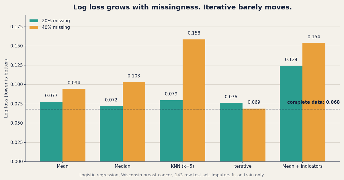
On complete data, logistic regression scored AUC 0.9977, accuracy 98.6% (141 of 143), log loss 0.0679. Here is what 20% missing did to it:
| Strategy | AUC | Accuracy | Log loss |
|---|---|---|---|
| Complete data | 0.9977 | 0.986 | 0.0679 |
| Mean | 0.9977 | 0.979 | 0.0772 |
| Median | 0.9975 | 0.986 | 0.0719 |
| KNN, k=5 | 0.9969 | 0.972 | 0.0794 |
| Iterative | 0.9966 | 0.965 | 0.0760 |
| Mean + indicators | 0.9868 | 0.937 | 0.1240 |
The four real imputers sit within 0.0011 of each other on AUC. Accuracy differs by at most four test rows. Log loss separates them a little: median is best at 0.0719, KNN worst at 0.0794, but the spread is small. At this missingness rate, arguing about imputation methods is arguing about noise. Pick the simplest one that your pipeline supports and spend the saved time checking whether the missingness is random in the first place.
The one exception is the indicator variant, which is clearly worse even at 20%: AUC 0.9868, accuracy 93.7%, log loss 0.1240. More on that in Finding 5.
Finding 3: at 40% missing, iterative imputation earns its keep
At 40% missing, the methods separate. Same model, same test set:
| Strategy | AUC | Accuracy | Log loss |
|---|---|---|---|
| Complete data | 0.9977 | 0.986 | 0.0679 |
| Mean | 0.9943 | 0.944 | 0.0940 |
| Median | 0.9941 | 0.944 | 0.1029 |
| KNN, k=5 | 0.9813 | 0.923 | 0.1583 |
| Iterative | 0.9987 | 0.972 | 0.0687 |
| Mean + indicators | 0.9868 | 0.937 | 0.1538 |
Iterative imputation at 40% missing scored AUC 0.9987 and log loss 0.0687. Compare that with complete data: AUC 0.9977, log loss 0.0679. The model trained on data that was 40% holes performed, for practical purposes, as well as the model trained on complete data. It got 139 of 143 test rows right, against 141 on complete data.
Why does it work here? Iterative imputation models each feature from all the others, and this dataset's features are heavily correlated. Mean radius, perimeter, and area correlate above 0.99 with each other (I measured those correlations in the feature-importance piece). When a value is missing, the other 29 features carry most of the information needed to reconstruct it. Mean imputation throws that information away. Iterative imputation uses it.
I checked this was not a one-seed fluke. With a different missingness seed, iterative at 40% scored AUC 0.9964 and log loss 0.0785. With a different train/test split, AUC 0.9954 and log loss 0.0865. In all three runs it was the best or tied-best method at 40%, and its log loss stayed within 0.02 of the complete-data figure. The headline holds.
Finding 4: KNN fades fastest as the holes multiply
KNN was competitive at 20% (AUC 0.9969, log loss 0.0794) and the worst method at 40% (AUC 0.9813, log loss 0.1583, accuracy 92.3%, or 132 of 143). Its log loss more than doubled between the two rates, while mean imputation's rose from 0.0772 to 0.0940.
The mechanism is straightforward. KNN fills a hole by averaging the nearest rows, but "nearest" is computed on rows that are themselves full of holes, using distances over whatever values happen to be present. At 20% missing, most rows still have enough observed values for the neighbourhood to mean something. At 40%, the neighbourhoods are built on guesses, and the guesses compound.
This is a useful general rule: any method whose input is other rows' observed values degrades faster than a method whose input is column statistics or a fitted model. KNN is the first of the three to feel it.
Finding 5: missing indicators hurt logistic regression here
Adding a binary "this value was missing" column per feature made logistic regression worse at both rates: AUC 0.9868 at 20% and 0.9868 at 40%, accuracy 93.7% in both cases, log loss 0.1240 and 0.1538. Mean imputation alone beat it on every metric at both rates.
That contradicts the scikit-learn user guide, which says adding a missingness indicator "tends to help prediction, even when values are missing completely at random." The guide is not wrong in general. Under MCAR, the indicator columns carry no signal by construction: whether a cell is missing is independent of everything, including the target. So the 30 extra binary columns are pure noise, and logistic regression fits weights on noise. On this dataset, with 426 training rows, that noise cost about a point of AUC and four test rows.
The random forest did not care. Its AUC with indicators was 0.9947 at 20% and 0.9895 at 40%, essentially tied with mean imputation. Trees can ignore useless columns by never splitting on them. Linear models cannot ignore a column; they assign it a coefficient and pay for it.
The lesson is narrower than "indicators are bad." Indicators help when missingness itself carries signal, which is common in real data: a missing lab value often means the doctor did not order the test, and that is informative. Under random missingness, indicators are noise columns, and linear models pay for noise. Know which case you are in before adding them.
Finding 6: the random forest barely notices
On complete data, the forest scored AUC 0.9949, accuracy 95.8%, log loss 0.1046. At 40% missing, its results by strategy:
| Strategy | AUC | Accuracy | Log loss |
|---|---|---|---|
| Complete data | 0.9949 | 0.958 | 0.1046 |
| Mean | 0.9886 | 0.958 | 0.1477 |
| Median | 0.9893 | 0.930 | 0.1510 |
| KNN, k=5 | 0.9802 | 0.923 | 0.1857 |
| Iterative | 0.9966 | 0.965 | 0.1064 |
| Mean + indicators | 0.9895 | 0.951 | 0.1594 |
Two things stand out. First, the forest's ranking of methods matches the logistic regression ranking: iterative best, KNN worst, indicators harmless. Second, the forest's accuracy barely moved at 20% (95.1% to 95.8% across methods, against 95.8% complete) and its best 40% result, iterative at 96.5%, actually beat its complete-data accuracy. Trees split on thresholds, so a mean-filled value lands on one side of a split or the other and the tree routes around it. The model's probability estimates suffer more than its hard predictions, which is why log loss moves more than accuracy.
If you are shipping a tree model and your missingness is moderate, imputation choice is a second-order concern. If you are shipping a linear model and your missingness is heavy, it is a first-order one.
What to do on Monday morning
- Count first, impute second. Before choosing a method, count what fraction of rows have any missing value. If it is above 90%, dropping rows is not an option, and any method that needs complete rows is not an option either.
- Under about 20% missing, use the mean or median and move on. On this data the four real methods were within 0.0011 AUC of each other. Your time is better spent checking whether the missingness is random.
- Over about 30% missing, try iterative imputation and compare it against the mean on a validation split. Here it recovered near-complete performance. It costs about a second on 426 rows and one extra import. That is cheap insurance.
- Do not add missingness indicators by default for linear models. Test them with and without. Under random missingness they are noise columns, and linear models pay for noise. Trees are more forgiving.
- Be careful with KNN imputation as missingness grows. It was fine at 20% and the worst method at 40%. If your missingness rate is high, KNN is the first method to distrust.
- Fit imputers on training data only, and apply them to test data. This sounds obvious and it is the easiest leak to introduce, because the imputer is usually built in the same notebook cell as the split. Put the imputer inside a pipeline so the rule enforces itself.
In favour
The design is clean: imputers fit on train only, test set holed the same way, two models, two rates, and the headline result reproduced across two extra seeds. The dataset's high feature correlations give iterative imputation a fair chance to show what it can do, and the drop-rows result is pure arithmetic that generalizes to any wide table.
Against
One dataset, one split, one missingness mechanism. The Wisconsin data is small, clean, and unusually correlated, which flatters iterative imputation and flatters the whole experiment. Accuracy differences of two or three test rows are within noise on a 143-row test set. And the indicator result directly contradicts the scikit-learn guide's general advice, which suggests my setup (pure MCAR, linear model, 30 noise columns) is a corner case, not a refutation.
What would make me wrong
- If iterative imputation loses to the mean on a dataset with weakly correlated features, the "use the other columns" explanation fails and the win here was dataset-specific.
- If a different missingness mechanism (missing at random, or not at random) flips the indicator result, then the Finding 5 warning applies only to MCAR and I overstated it.
- If KNN with a larger k, or with distance weighting, holds up at 40%, then the fade I measured is a k=5 artifact, not a KNN property.
- If a proper cross-validated comparison shows the 20% differences are all noise, then Finding 2's "barely matters" becomes "does not matter at all," which only strengthens the practical advice.
Key takeaways
- Dropping rows with missing values is not viable on wide tables: at 20% missing across 30 features, 425 of 426 rows had a hole.
- At 20% missing, mean, median, KNN, and iterative imputation performed within 0.0011 AUC of each other for logistic regression. Use the simplest one.
- At 40% missing, iterative imputation recovered near-complete performance (AUC 0.9987, log loss 0.0687 vs 0.9977 and 0.0679 complete), while KNN fell to AUC 0.9813 and log loss 0.1583.
- Missingness indicators hurt logistic regression under random missingness (AUC 0.9868 vs 0.9943 for mean alone at 40%) because they add 30 noise columns. Trees were unaffected.
- Random forests are robust to imputation choice: accuracy stayed between 95.1% and 95.8% at 20% missing across all methods, and iterative imputation at 40% beat the complete-data accuracy.
When did you last check what fraction of your rows actually survive a dropna()? If the answer is "never," run it today. You might find your dataset is thinner than you think.
Related on Everyday Data Science: Scaling Gave SVM 8 Points and Trees Nothing. I Ran Four Models Raw and Scaled. · 98% Accurate and Useless: Six Imbalance Fixes, Measured on a 2% Positive Class · Three Rankings, One Model, Little Agreement: Feature Importance Is a Question, Not a Number
Sources: scikit-learn user guide, Imputation of missing values · scikit-learn, load_breast_cancer
About the writer
Data Scientist & AI Researcher
Data scientist and AI researcher at Pace University. I coined Artificial Frictional Unemployment, and built the first machine learning model for crop yield prediction in Sierra Leone. Author of Understanding Agentic AI. I write about agentic systems and applied ML, with a bias toward what actually works, and who gets left out when it doesn't.
Found this useful? Passing it on to someone who builds is the best way to help the publication grow.
Built something worth sharing? Write it up for us →