Scaling Gave SVM 8 Points and Trees Nothing. I Ran Four Models Raw and Scaled.
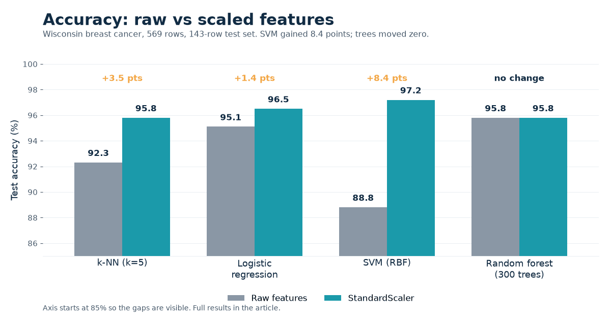
Four models, one breast-cancer dataset, raw features vs StandardScaler: k-NN gained 3.5 points, SVM gained 8.4, logistic regression finally converged, and random forest did not move at all.
 Ibrahim Denis FofanahData Scientist & AI Researcher10 min read·From Notebook to Production · Explainer
Every tutorial tells you to scale your features. Few of them show you what happens if you do not, in numbers, on the same data, with the same code. So I ran the comparison. Four models, one dataset, raw versus scaled, plus one deliberate trap: a single feature multiplied by 1,000.
The setup
The dataset is the Wisconsin breast-cancer set that ships with scikit-learn: 569 rows, 30 numeric features measured from cell nuclei, 212 malignant and 357 benign. I used a stratified 75/25 split with seed 42, which leaves a 143-row test set. One test row is worth 0.7 points of accuracy, so keep that in mind when you read the gaps below.
The four models ran with near-default settings in scikit-learn 1.9.1: k-NN with k=5, logistic regression with max_iter=1000, an RBF-kernel SVM, and a random forest with 300 trees. The only preprocessing was StandardScaler, fit on the training set and applied to the test set, exactly as the docs prescribe. Nothing else changed between the two runs.
from sklearn.datasets import load_breast_cancer
from sklearn.model_selection import train_test_split
from sklearn.preprocessing import StandardScaler

X, y = load_breast_cancer(return_X_y=True)
X_train, X_test, y_train, y_test = train_test_split(
    X, y, test_size=0.25, random_state=42, stratify=y)

scaler = StandardScaler().fit(X_train)   # fit on train only
X_train_s = scaler.transform(X_train)
X_test_s = scaler.transform(X_test)
The scale gap in the raw data
Before any model ran, the raw features already told the story. Feature means in this dataset run from 0.0038 to 880.58, a spread of more than 200,000 times. The largest feature, worst area, averages 880.58. Mean radius averages 14.13. Standard deviations run from 0.0026 to 568.86. That is not a subtle difference in units. It is the difference between a feature that whispers and a feature that shouts, and any model that measures distance will listen to the shouter first.
| feature | mean | standard deviation |
|---|---|---|
| smallest feature mean | 0.0038 | 0.0026 |
| mean radius | 14.13 | 3.52 |
| worst area | 880.58 | 568.86 |
The results
| model | raw accuracy | scaled accuracy | change | raw F1 (malignant) | scaled F1 (malignant) |
|---|---|---|---|---|---|
| k-NN (k=5) | 92.3% | 95.8% | +3.5 | 0.887 | 0.941 |
| Logistic regression | 95.1% | 96.5% | +1.4 | 0.931 | 0.952 |
| SVM (RBF) | 88.8% | 97.2% | +8.4 | 0.822 | 0.961 |
| Random forest (300 trees) | 95.8% | 95.8% | 0.0 | 0.940 | 0.940 |
F1 is reported with malignant as the positive class. The headline is the SVM column, but each row has its own lesson.
Finding 1: SVM was the biggest winner, by far
The RBF SVM went from 88.8% to 97.2%, a gain of 8.4 points, or 12 more correct rows out of 143. Its F1 for the malignant class rose from 0.822 to 0.961. On raw features it was the worst model in the test. On scaled features it was the best, by a clear margin.
The mechanism is not mysterious. An RBF kernel measures distance between rows, and distance is dominated by the largest-scale features. With worst area averaging 880 and other features averaging under 1, the kernel was effectively comparing rows on one or two features and ignoring the rest. Scaling put every feature on the same footing, and the kernel could finally use all 30 of them. The 8.4-point gain is what 28 ignored features are worth.
Finding 2: k-NN gained 3.5 points, and it was not a lucky split
k-NN moved from 92.3% to 95.8%, five more correct rows, and its F1 rose from 0.887 to 0.941. Same mechanism as the SVM: nearest neighbours are computed in Euclidean distance, and raw distances were dominated by the big features.
Because a single split can flatter a result, I re-ran k-NN on five split seeds, raw and scaled each time. Scaling won on all five.
| split seed | k-NN raw | k-NN scaled |
|---|---|---|
| 42 | 92.3% | 95.8% |
| 0 | 92.3% | 93.7% |
| 1 | 92.3% | 95.8% |
| 2 | 93.7% | 95.1% |
| 3 | 92.3% | 98.6% |
| mean | 92.6% | 95.8% |
The mean gap is 3.2 points, and the direction never flipped. The single-seed result was not a fluke. It was the middle of the distribution.
Finding 3: logistic regression did not just get more accurate, it finally converged
This is the finding I did not expect. On raw features, logistic regression burned through all 1,000 allowed iterations and still raised a ConvergenceWarning. Its reported accuracy, 95.1%, came from a model that never finished optimizing. On scaled features it converged in 20 iterations, no warning, and scored 96.5%.
The fit time tells the same story: 0.504 seconds raw, 0.018 seconds scaled, about 28 times faster. Gradient descent on unscaled features takes tiny steps in some directions and huge ones in others, so it crawls. Scaling makes the loss surface roughly round, and the optimizer walks straight to the answer.
The honest way to state the raw result is that it is not a measurement you can lean on. A model that hits its iteration cap has not solved the problem you gave it. If you see a ConvergenceWarning in your own work, scaling is the first thing to try before you reach for a larger max_iter.
Finding 4: trees did not notice at all
Random forest scored 95.8% raw and 95.8% scaled, with F1 of 0.940 both ways, identical to four decimal places. Fit time moved from 0.65 to 0.79 seconds, which is noise on a job this small.
That is exactly what theory predicts. A tree splits on one feature at a time, comparing values of that feature against a threshold. Multiplying a feature by 1,000 moves the threshold by the same factor and changes nothing about which rows fall on which side. Scaling is a monotone transform per feature, and trees are invariant to monotone transforms. If your pipeline is trees all the way down, scaling is wasted compute. If it is not, scaling is the cheapest accuracy you will ever buy.
The trap: one feature, multiplied by 1,000
The last test asked a narrower question. Suppose 29 of your features are fine and one arrives in the wrong units, say millimetres instead of metres, or a raw count where everything else is a rate. I multiplied mean radius by 1,000 in both train and test and re-ran all four models.
| model | raw accuracy | one feature x1,000 | change |
|---|---|---|---|
| k-NN (k=5) | 92.3% | 89.5% | -2.8 |
| Logistic regression | 95.1% | 95.8% | +0.7 |
| SVM (RBF) | 88.8% | 86.7% | -2.1 |
| Random forest (300 trees) | 95.8% | 95.8% | 0.0 |
k-NN lost 2.8 points and SVM lost 2.1, because one inflated feature now dominated every distance they computed. Random forest, again, did not move. Logistic regression ticked up slightly to 95.8%, but it still failed to converge in 1,000 iterations, so that number is a non-converged model beating another non-converged model by one row, and I would not build anything on it.
The point of the trap is how little it takes. One column in the wrong units cost the distance models two to three points, silently. No error, no warning, just a worse model.
Why it works, in one paragraph
Distance-based models (k-NN, RBF SVM) and gradient-based models (logistic regression, neural nets) treat the raw numbers as geometry. A feature that ranges over hundreds counts hundreds of times more than a feature that ranges over fractions, regardless of which one carries signal. Scaling re-expresses every feature in units of its own spread, so a one-standard-deviation move means the same thing everywhere. Tree models split one feature at a time and never compare features against each other, so they are immune. That single distinction, distance versus splits, predicts every number in this article.
What to do with this
- Scale before any distance or gradient model: k-NN, SVM, logistic regression, neural nets, k-means, PCA. Do it by default and stop debating it per project.
- Fit the scaler on the training set only, then transform the test set. Fitting on all the data leaks test information into training, and it is the same class of mistake as the pre-split feature selection I measured in October.
- Treat a ConvergenceWarning as a scaling problem first. If your logistic regression or SVM warns, scale before you raise max_iter.
- Skip scaling for pure tree pipelines. It costs nothing to do, but it buys nothing either, and a step that buys nothing is a step that can break.
- Re-check your scales every time you add a feature. One new column in the wrong units cost my distance models two to three points with no error message. A one-line summary of feature means and standard deviations, printed before training, catches it.
In favour
Scaling is free, it is one line, and it cannot hurt a distance model. The theory behind it is settled, and the measured gains here point the same way on every model the theory predicts. The convergence finding is the strongest kind of evidence for a practitioner: a warning disappeared and the fit got 28 times faster.
Against
One dataset is one dataset. Breast-cancer features are all positive, continuous, and roughly bell-shaped, which is friendly territory for StandardScaler. Heavily skewed features, outliers, or sparse data can make standardization the wrong scaler, and RobustScaler or a log transform may be the right call instead. The test set is small, so the 1.4-point logistic regression gain is within the noise of a couple of rows. And the raw SVM score of 88.8% is partly a story about default hyperparameters: tuning C and gamma on raw features would close some of that gap, though it would not fix the underlying geometry.
What would make me wrong
Run the same comparison on a dataset where features are already on similar scales and the gaps should shrink to near zero. Run it on a dataset with one extreme outlier and StandardScaler should underperform RobustScaler. Re-run the SVM comparison with a tuned C and gamma on raw features: if the raw score climbs to 97%, the lesson becomes "tune your model" rather than "scale your features", and I would have overstated the scaler. The convergence claim is the easiest to falsify: find a logistic regression that converges in 20 iterations on raw features with a 200,000-to-1 scale spread, and the mechanism I described is wrong.
Key takeaways
- SVM gained 8.4 points from one preprocessing line, 88.8% to 97.2%, because its kernel could finally use all 30 features.
- k-NN gained 3.5 points and won on all five split seeds, mean 92.6% raw versus 95.8% scaled.
- Logistic regression on raw features never converged in 1,000 iterations. Scaled, it converged in 20 and fit 28 times faster.
- Random forest scored 95.8% both ways, identical to four decimals. Trees do not care about scale.
- One feature multiplied by 1,000 cost k-NN 2.8 points and SVM 2.1, silently. Check your scales when you add a feature.
When did scaling last change a result of yours, and did you notice it at the time or only in hindsight?
Related on Everyday Data Science:
- Five Leaks That Inflate Your AUC: I Measured Each One
- Same Model, Ten Seeds, a 3.5-Point Swing: Why One Split Is Not a Result
- Your 0.85 Meant 0.98: A 20,000-Row Calibration Test That Caught a Top Model Misstating Its Own Odds
Sources: scikit-learn load_breast_cancer docs, scikit-learn preprocessing user guide, StandardScaler reference. All numbers are from my own runs, scikit-learn 1.9.1, code and results in the article.
Drift Is Three Different Failures, and One Metric Cannot See Them All
Next →Your 0.85 Meant 0.98: A 20,000-Row Calibration Test That Caught a Top Model Misstating Its Own Odds
About the writer
Data Scientist & AI Researcher
Data scientist and AI researcher at Pace University. I coined Artificial Frictional Unemployment, and built the first machine learning model for crop yield prediction in Sierra Leone. Author of Understanding Agentic AI. I write about agentic systems and applied ML, with a bias toward what actually works, and who gets left out when it doesn't.
Found this useful? Passing it on to someone who builds is the best way to help the publication grow.
Built something worth sharing? Write it up for us →