Drift Is Three Different Failures, and One Metric Cannot See Them All
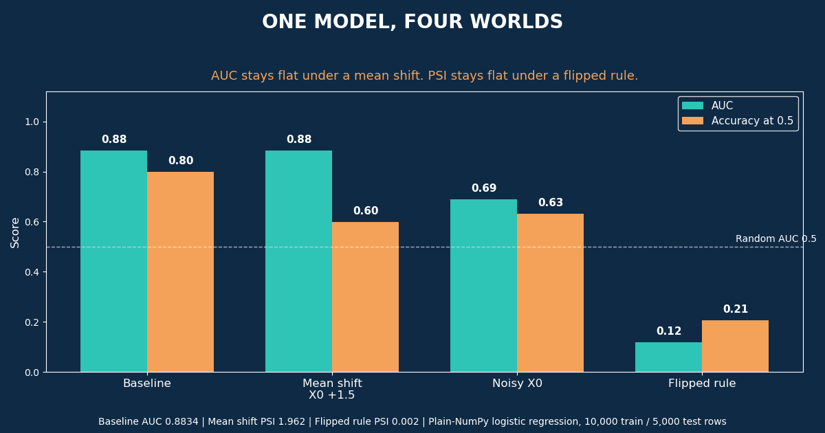
A mean shift left AUC exactly unchanged while accuracy fell from 0.80 to 0.60. A flipped labeling rule scored AUC 0.12 while PSI read 0.002. Every drift metric is blind to something, so a monitoring setup needs more than one.
 Ibrahim Denis FofanahData Scientist & AI Researcher9 min read·From Notebook to Production · Explainer
Production models rarely fail the way a test set suggests. The test set is frozen. Production is not. Inputs change, the meaning of a label changes, and sometimes both change at once, and each kind of change breaks a different part of your evaluation. Teams that watch one number learn this late, usually from a business metric, not from their dashboard.
This piece separates the three failures, measures each one on the same model, and shows exactly which metric catches which failure and which one misses it.
The three kinds of drift
Drift is a change in the joint distribution of inputs X and labels y. The standard split, used in the concept drift literature, separates it by what changed:
- Covariate shift (data drift): P(X) changes, P(y given X) stays the same. The inputs move, but a given input still means what it meant. Example: a loan model trained on one age mix starts seeing a younger applicant mix.
- Concept drift: P(y given X) changes. The same inputs now mean something different. Example: a fraud pattern that once signaled stolen cards becomes normal shopping behavior. This is the hardest kind, because the inputs alone show nothing wrong.
- Label drift (prior probability shift): P(y) changes. The base rate of outcomes moves, so probabilities anchored to the old base rate are miscalibrated even if the ranking is fine.
These types are not mutually exclusive, and in real systems they often arrive together. The experiment below isolates them on purpose, because isolation is the only way to learn what each metric can and cannot see.
The experiment
The setup is synthetic and fully specified, so every number below can be reproduced. Two features, X0 and X1, drawn from a standard normal distribution. The true labeling rule is logit = 2.0 times X0 minus 1.0 times X1, with labels sampled from that probability. I trained a logistic regression model in plain NumPy on 10,000 rows (seed 42). Its fitted weights, 1.93 and minus 1.02 with a bias of 0.02, are close to the true rule, which is the point: this is a good model on its training distribution, not a broken one.
Then I scored it on four 5,000-row test sets:
- Baseline: same distribution as training.
- Mean shift: the same labels, but X0 increased by 1.5 for every test row. Same rule, moved inputs. Pure covariate shift.
- Noisy feature: the same labels, but Gaussian noise with standard deviation 2.0 added to X0. Same rule, degraded inputs.
- Flipped rule: the same inputs, but labels generated by the opposite rule, logit = minus 2.0 times X0 plus 1.0 times X1. Pure concept drift.
PSI on X0 was computed with 10 quantile bins from the training distribution. The standard rule of thumb bands are PSI below 0.1 for little change, 0.1 to 0.25 for moderate change, and 0.25 or above for significant change.
def psi(expected, actual, bins=10):
    qs = np.quantile(expected, np.linspace(0, 1, bins + 1))
    qs[0] -= 1e-6
    qs[-1] += 1e-6
    e, _ = np.histogram(expected, bins=qs)
    a, _ = np.histogram(actual, bins=qs)
    e = np.maximum(e / len(expected), 1e-4)
    a = np.maximum(a / len(actual), 1e-4)
    return float(np.sum((a - e) * np.log(a / e)))
The results
| Scenario | AUC | Accuracy at 0.5 | Log loss | Predicted positive rate | PSI on X0 |
|---|---|---|---|---|---|
| Baseline, same distribution | 0.8834 | 0.7978 | 0.4271 | 0.5102 | 0.002 |
| Mean shift, X0 + 1.5 | 0.8834 | 0.5974 | 0.9643 | 0.9126 | 1.962 |
| Noisy X0, added N(0, 2) | 0.6885 | 0.6312 | 1.1818 | 0.4936 | 0.436 |
| Flipped rule, same inputs | 0.1201 | 0.2060 | 1.8116 | 0.5102 | 0.002 |
Read the table row by row, because each row embarrasses a different metric.
The mean shift row is the quiet one. AUC is identical to baseline, to four decimal places: 0.8834 in both cases. That is not a rounding coincidence. Adding a constant to every test row's X0 shifts every score by the same amount, so the ranking of cases is untouched, and AUC measures ranking only. But accuracy at the fixed 0.5 threshold fell from 0.7978 to 0.5974, the predicted positive rate jumped from 0.5102 to 0.9126, and log loss more than doubled, from 0.4271 to 0.9643. The model still ranks perfectly well. It now calls almost everything positive, and its probabilities are wrong. A dashboard that shows AUC alone would report no problem while the threshold rule downstream approves nearly everyone.
PSI, to its credit, screams here: 1.962, far above the 0.25 significant-change band. Input monitoring catches what AUC misses, in this row.
The noisy feature row is the honest degradation. AUC fell to 0.6885, accuracy to 0.6312, log loss rose to 1.1818, and PSI read 0.436, again above the significant band. Every metric agrees something is wrong. Noise destroys information, and no threshold trick recovers it. The fix here is upstream: find why the feature degraded, or drop it, rather than retraining on noisy inputs and hoping.
The flipped rule row is the dangerous one. AUC collapsed to 0.1201, below random guessing, because the model now ranks the world backwards. Accuracy fell to 0.2060. Log loss rose to 1.8116. And PSI read 0.002, the same as baseline. The inputs did not move at all, so any input-only monitor, PSI, distribution tests, range checks, would report a healthy system while the model is actively wrong. Concept drift is invisible to input monitoring by definition. The only signals that catch it are labeled outcomes, or proxies for them: rising error rates on audited labels, rising human override rates, or a business metric moving against the model's predictions.
What each metric can and cannot see
- AUC sees ranking, nothing else. It is blind to pure mean shifts and to calibration failure. Use it to check whether the model still orders cases correctly.
- Accuracy at a fixed threshold sees threshold damage. It caught the mean shift that AUC missed. But it needs labels, and it hides calibration damage behind a single cutoff.
- Log loss sees probability quality. It rose in every drift row, including the mean shift row where AUC was flat. If your decisions multiply probabilities by costs, log loss is the metric that matters, and it needs labels too.
- PSI sees input distribution change, nothing else. It caught both input shifts with large margins, 1.962 and 0.436, and it was blind to concept drift, 0.002. PSI needs no labels, which is why it runs first in production. That convenience is also its limit.
- Predicted positive rate is a free early warning. It needs no labels either. In the mean shift row it jumped from 0.5102 to 0.9126, a change any alerting rule would catch. In the flipped rule row it did not move, 0.5102, which is itself informative: a stable prediction mix with worsening outcomes points at concept drift, not at input drift.
The verdict
A monitoring setup built on one metric will miss at least one kind of drift, guaranteed, because the failure modes are complementary by construction. The minimum viable setup from this experiment is four signals, not one:
- Input PSI or distribution tests on key features, no labels needed. Catches covariate shift early. Alert above 0.25, investigate above 0.1 on a critical feature.
- Predicted class and score distribution, no labels needed. Catches threshold damage and gives a free daily signal. A stable mix with worsening business outcomes points at concept drift.
- Performance on fresh labeled data, on a schedule, even a small audited sample. This is the only signal that catches concept drift. Without it, you are guessing.
- Log loss or calibration error alongside AUC. AUC alone will tell you the ranking is fine while the probabilities are wrong, and probabilities are what thresholds, triage queues, and expected-value calculations actually use.
And the response differs by diagnosis. Covariate shift may need recalibration, a threshold move, or retraining on the new mix. Noisy inputs need an upstream fix. Concept drift needs fresh labels and a new model, because no amount of threshold tuning repairs a flipped rule. Retraining on stale labels under concept drift just re-learns the old world faster.
Key takeaways
- AUC measures ranking only. A pure mean shift leaves it exactly unchanged while accuracy falls 0.20 points.
- PSI measures input distribution only. It read 1.962 for a mean shift and 0.002 for a flipped rule that destroyed the model.
- A predicted positive rate jump, 0.51 to 0.91 here, is a label-free alarm that catches threshold damage AUC misses.
- Concept drift is invisible without labels or label proxies. Budget for an audited labeled sample, or accept that you will learn about it from business damage.
- Log loss rose in every drift scenario. If decisions use probabilities, track it next to AUC, not instead of it.
- Diagnose before retraining. The fix for a shifted input, a noisy feature, and a flipped rule are three different actions, and the wrong one wastes a retrain.
Which metric has misled you the most in production: a ranking score that stayed green, an input monitor that stayed quiet, or a threshold that silently moved? Tell me which one, and what finally caught it.
Related on Everyday Data Science
- Five Leaks That Inflate Your AUC: I Measured Each One
- Your 0.85 Meant 0.98: A 20,000-Row Calibration Test That Caught a Top Model Misstating Its Own Odds
- Most Analytics Bugs Are Data Bugs. Five Checks That Catch Them Before the Meeting.
Sources: Population Stability Index thresholds, Towards Data Science, PSI interpretation bands, Arize, concept drift and covariate shift definitions, Towards Data Science, drift types and detection, Safeguard
Five Leaks That Inflate Your AUC: I Measured Each One
Next →Your 0.85 Meant 0.98: A 20,000-Row Calibration Test That Caught a Top Model Misstating Its Own Odds
About the writer
Data Scientist & AI Researcher
Data scientist and AI researcher at Pace University. I coined Artificial Frictional Unemployment, and built the first machine learning model for crop yield prediction in Sierra Leone. Author of Understanding Agentic AI. I write about agentic systems and applied ML, with a bias toward what actually works, and who gets left out when it doesn't.
Found this useful? Passing it on to someone who builds is the best way to help the publication grow.
Built something worth sharing? Write it up for us →