Your 0.85 Meant 0.98: A 20,000-Row Calibration Test That Caught a Top Model Misstating Its Own Odds

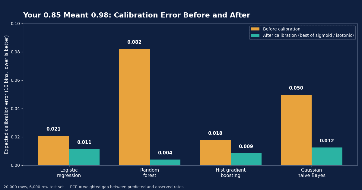
A model that outputs 0.85 is making a numerical claim: out of 100 cases scored like this one, about 85 should be positive. Most teams never check that claim. They check AUC, they check accuracy at 0.5, and then they ship the raw score into a threshold rule, a triage queue, or an expected-value calculation that treats 0.85 as 85%.

That is where the damage happens. A ranking can be excellent while the numbers attached to it are wrong, in either direction, and any decision that multiplies a probability by a cost, a price, or a capacity limit inherits the error in full.

I ran a controlled test to measure how large that error is for the classifiers practitioners reach for most, and how much of it a standard post-hoc fix actually removes.

The setup

The data is synthetic and fully specified, so anyone can reproduce every number in this piece: make_classification with 20,000 rows, 20 features (12 informative, 4 redundant), a 72/28 class split, 2% label noise, and random_state=42, generated with scikit-learn 1.9.1. The split was 14,000 rows for training and 6,000 for testing, stratified, with a 28.5% positive rate in the test set.

Four models, all with default or near-default settings:

1. Logistic regression
2. Random forest, 300 trees
3. HistGradientBoostingClassifier
4. Gaussian naive Bayes

Each model was scored three ways on the same test set: raw, after sigmoid (Platt) calibration, and after isotonic calibration, both fitted with CalibratedClassifierCV using 3-fold cross-validation on the training data. Calibration error is expected calibration error (ECE) with 10 equal-width bins: bin the predictions, compare the mean predicted probability in each bin with the observed positive rate, and average the gaps weighted by bin size. I also report Brier score, log loss, and AUC.

The results

Model	AUC, raw	Brier, raw	Brier, calibrated (best)	ECE, raw	ECE, sigmoid	ECE, isotonic
Logistic regression	0.8860	0.1193	0.1188 (isotonic)	0.0208	0.0217	0.0113
Random forest	0.9718	0.0553	0.0451 (sigmoid)	0.0821	0.0039	0.0074
Hist gradient boosting	0.9722	0.0437	0.0415 (isotonic)	0.0178	0.0112	0.0085
Gaussian naive Bayes	0.8809	0.1278	0.1223 (isotonic)	0.0498	0.0384	0.0124

Three findings matter.

1. The best-ranking model was the worst calibrated

Random forest and gradient boosting ranked cases almost identically (AUC 0.9718 and 0.9722) and far ahead of the other two models. On calibration they were nowhere near each other: gradient boosting posted the lowest raw ECE in the test at 0.0178, while the random forest posted the highest at 0.0821, more than four times worse.

AUC cannot detect this gap. AUC only asks whether positives tend to score higher than negatives. A model can pass that test with the best score in the room while its stated probabilities are off by eight points on average.

2. The forest was underconfident, not overconfident

The usual warning is that models claim too much certainty. This forest did the opposite in its middle and upper bins:

Random forest bin (raw)	Cases	Mean prediction	Actually positive
0.5 to 0.6	205	0.550	73.7%
0.6 to 0.7	283	0.654	87.6%
0.7 to 0.8	368	0.756	97.8%
0.8 to 0.9	401	0.852	97.8%
0.9 to 1.0	343	0.947	98.3%

Averaging trees compresses probabilities away from the extremes, and here that compression badly understated how separable the upper range was. A team triaging by this score would have treated near-certain cases as coin-flip-adjacent. After sigmoid calibration, ECE fell from 0.0821 to 0.0039, Brier score from 0.0553 to 0.0451, and log loss from 0.2235 to 0.1691.

Direction matters less than the habit of checking. Overconfidence and underconfidence both corrupt any decision that uses the number, and you cannot tell which one your model has from AUC.

3. There was no universal winning calibrator

Isotonic calibration gave the best ECE for three of the four models: logistic regression (0.0208 down to 0.0113), gradient boosting (0.0178 down to 0.0085), and Gaussian naive Bayes (0.0498 down to 0.0124, with log loss down from 0.4192 to 0.3874). But for the random forest, sigmoid calibration won clearly (0.0039 against isotonic at 0.0074), because the forest's distortion was smooth and close to the sigmoid shape that Platt scaling assumes.

Logistic regression is the honest middle case. It was not the best calibrated model raw, that was gradient boosting, but calibration still halved its ECE under isotonic fitting while sigmoid fitting made it slightly worse (0.0217). Even a well-behaved model deserves the check, and even for it, the choice of calibrator matters.

What calibration actually does

Both methods used here learn a mapping from raw scores to corrected probabilities on data the base model did not train on, which is why CalibratedClassifierCV fits the mapping with cross-validation rather than on training predictions the model has already memorized.

• Sigmoid (Platt) scaling fits a two-parameter logistic curve. It assumes the distortion has a sigmoid shape. It is stable on small calibration sets because there is little to overfit, and it was the best fix for the random forest here.
• Isotonic regression fits any monotonic step function. It makes no shape assumption, which is why it won on the other three models, but it needs enough held-out data to estimate those steps without memorizing noise.

For neural networks, the standard fix is a close relative. Guo and co-authors (ICML 2017, arXiv:1706.04599) showed that modern deep networks tend to be overconfident, and that temperature scaling, a one-parameter variant of Platt scaling applied to logits, corrected much of the error in their tests. The principle is identical: keep the model, fix the meaning of its output on held-out data.

One property deserves precision. Because these calibrators are monotonic, they should preserve ranking, and in this test AUC moved by at most 0.001 in any direction (random forest sigmoid: 0.9711 against 0.9718 raw; gradient boosting sigmoid actually ticked up to 0.9728). The small movements come from CalibratedClassifierCV refitting the base model inside its cross-validation folds. The practical point stands: if your model ranks badly, calibration will not save it. It will only make its ranking sound more precise.

When this matters, and when it does not

Calibration matters when the number itself enters a decision:

• A threshold set from costs, such as reviewing a transaction when expected fraud loss exceeds review cost
• Triage and queue priority, where a 0.90 case is meant to be worked before a 0.60 case because it is genuinely more likely
• Combining a model probability with money, capacity, or risk limits
• Reporting a risk figure to a clinician, lender, or regulator who will read 0.85 as 85%

It matters much less when only the order is used: a top-100 list, a retrieval ranking, or a fixed-capacity review queue that works down from the highest score. There, spend the effort on ranking quality instead.

A practical checklist

1. Plot a reliability diagram and compute ECE before you ship any score that will be read as a probability. State your bin count when you report ECE, because the number depends on it.
2. Try both sigmoid and isotonic calibration and keep the one that scores better on held-out data. In this test the winner changed by model.
3. With a small held-out set, prefer sigmoid scaling. With thousands of held-out rows, isotonic has the data it needs to beat it, as it did for three of four models here.
4. Never fit the calibrator on the same predictions the model produced for its own training rows. Use cross-validated out-of-fold predictions or a dedicated calibration set.
5. Judge the fix on Brier score and log loss as well as ECE. In this test all three moved together for the badly calibrated models, which is the signal that the improvement is real and not an artifact of binning.
6. Put a recalibration check in monitoring, next to the drift checks you already run.

The verdict

Raw probabilities should not be read at face value, even from your best model, especially from your best model. In this test the top-ranked classifier misstated its own odds by 0.082 on average, and a standard calibration step removed nearly all of that error at no meaningful cost to ranking. The check takes minutes. Skipping it means every threshold, triage rule, and expected-value calculation downstream is built on a number nobody verified.

Key takeaways

1. AUC measures ranking only. Two models tied at AUC 0.972 differed by more than four times on calibration error (0.0178 vs 0.0821).
2. The random forest was underconfident: its 0.8 to 0.9 bin averaged 0.852 predicted and delivered 97.8% positives.
3. Sigmoid calibration fixed the forest (ECE 0.0821 to 0.0039); isotonic calibration won for the other three models. Test both.
4. Gaussian naive Bayes improved from ECE 0.0498 to 0.0124 and log loss from 0.4192 to 0.3874 under isotonic calibration.
5. Calibration moved AUC by at most 0.001 in this test. It fixes what a score means, not how well a model separates classes.
6. Calibration expires under drift. Recheck and refit it like any other production component.

What would make me wrong

The forest's underconfidence may be specific to this synthetic setup, where the informative features create well-separated clusters that tree averaging compresses. On messier real data, the same model class often errs in the opposite direction, toward overconfidence, and the headline bin in this piece would flip sign. The broader claim, that raw probabilities need checking because the error can be large in either direction, would survive that flip; the specific numbers would not transfer. ECE with 10 uniform bins can also hide miscalibration inside sparse bins, and a quantile-binned check on the same predictions is the follow-up I would run before quoting these gaps in a production postmortem. Finally, with a 500-row calibration set I would expect sigmoid scaling to win more often, because isotonic fitting needs data to estimate its steps.

When did a raw model probability last cost you a bad decision, and did you catch it from a reliability diagram or from the decision itself?

Related on Everyday Data Science:

• Pandas vs Polars vs DuckDB on 3.5M rows
• Tabular Foundation Models vs Gradient Boosting
• Five Data Validation Checks

Sources

• Guo, Pleiss, Sun and Weinberger, On Calibration of Modern Neural Networks, arXiv:1706.04599
• scikit-learn user guide, Probability calibration
• scikit-learn example, Probability calibration of classifiers
• Niculescu-Mizil and Caruana, Predicting Good Probabilities With Supervised Learning, ICML 2005, DOI: 10.1145/1102351.1102430

All experimental numbers in this article are from the author's own run described in the setup section: scikit-learn 1.9.1, 20,000 synthetic rows, random_state=42, 6,000-row test set.